Centrality Measures
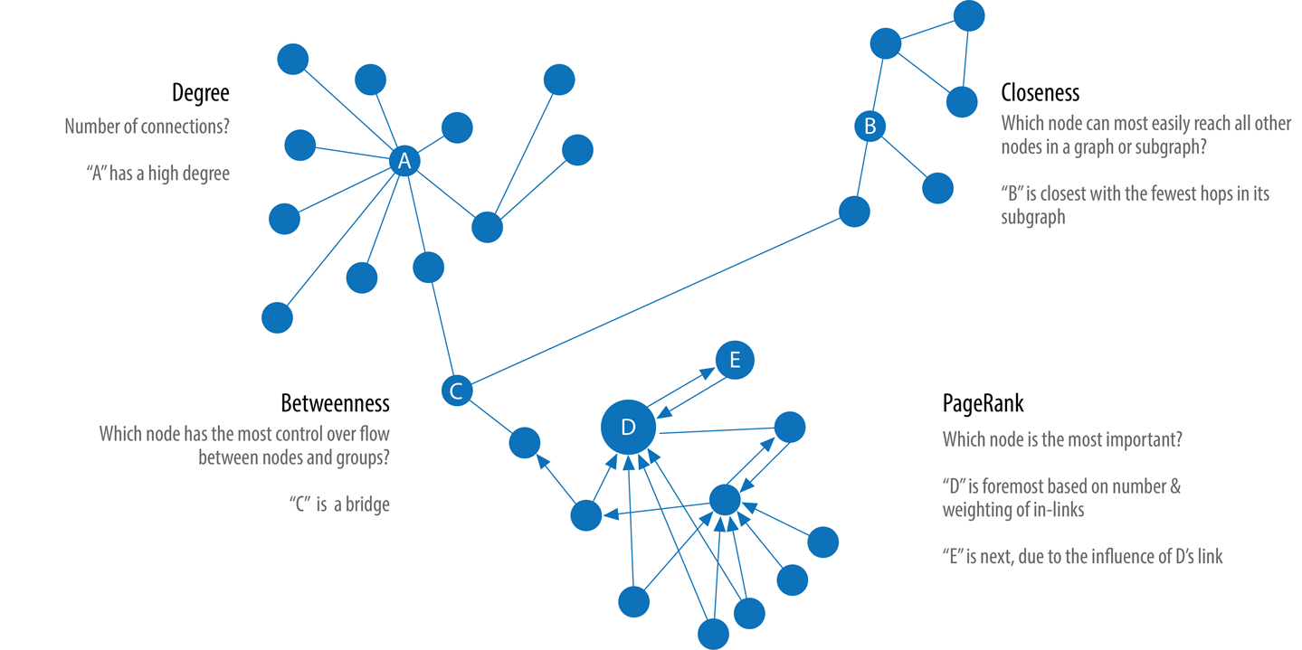
Centrality algorithms are used to understand the roles of particular nodes in a graph and their impact on that network.
Degree Centralityas a baseline metric of connectednessCloseness Centralityfor measuring how central a node is to the groupBetweenness Centralityfor finding control pointsPageRankfor understanding the overall influence
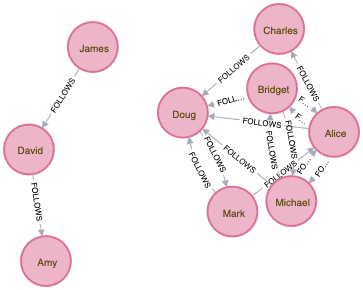
Example Graph Data: A Social network
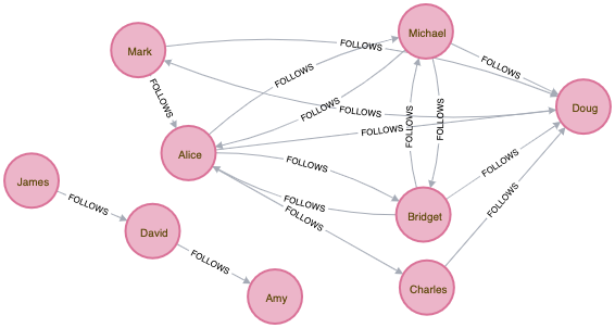
Centrality algorithms are relevant to all graphs, but social networks provide a very relatable way to think about dynamic influence and the flow of information. The examples in this chapter are run against a small Twitter-like graph. You can download the nodes and relationships csv-files we’ll use to create our graph.
Nodes : social-nodes.csv
Relationships : social-relationships.csv
After creating the database we can read the csv files using our Cypher commands :
WITH "file:///social-nodes.csv"
AS data
LOAD CSV WITH HEADERS FROM data AS row
MERGE (:User {id: row.id})
WITH "file:///social-relationships.csv"
AS data
LOAD CSV WITH HEADERS FROM data AS row
MATCH (source:User {id: row.src})
MATCH (destination:User {id: row.dst})
MERGE (source)-[:FOLLOWS]->(destination)
Degree Centrality
The degree counts the number of incoming and outgoing relationships from a node, and is used to find popular nodes in a graph. Degree Centrality was proposed by Linton C. Freeman (1979) For example, a person with a high degree in an active social network would have a lot of immediate contacts and be more likely to catch a cold circulating in their network.
The average degree of a network is simply the total number of relationships divided by the total number of nodes. This can be heavily skewed by high degree nodes. The degree distribution is the probability that a randomly selected node will have a certain number of relationships.
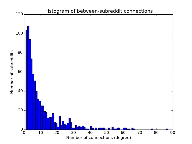
The graph above shows that the average degree is 10. But the median is 2. This illustrates the heavily skewed nature of a some networks. (ref: Jacob Silterra)
When Should I Use Degree Centrality?
Use Degree Centrality if you’re attempting to analyze influence by looking at the number of incoming and outgoing relationships, or find the “popularity” of individual nodes.
To get the nodes that are following most other users can be done very easily in Neo4j.
First create our graph and give it the name social:
CALL gds.graph.create('social','USER','FOLLOWS')
CALL gds.degree.stream('social')
YIELD nodeId, score
RETURN gds.util.asNode(nodeId).id AS name, score AS followers
ORDER BY followers DESC
Note that it is not required to use a graph from the graph catalog:
CALL gds.degree.stream({
nodeProjection: 'User',
relationshipProjection: {FOLLOWS: {type: 'FOLLOWS'}}})
YIELD nodeId, score
RETURN gds.util.asNode(nodeId).id AS name, score AS followers
ORDER BY followers DESC
name |
followers |
|---|---|
Alice |
4.0 |
Bridget |
3.0 |
Michael |
3.0 |
Mark |
2.0 |
Charles |
1.0 |
Doug |
1.0 |
David |
1.0 |
James |
1.0 |
Amy |
0.0 |
It is also possible to store the results as properties of the different nodes :
CALL gds.degree.write({
nodeProjection: 'User',relationshipProjection:
{FOLLOWS: {type: 'FOLLOWS'}},writeProperty:'followers'})
MATCH (n:User)
RETURN n.id as name, n.followers as followers
name |
followers |
|---|---|
Alice |
4.0 |
Bridget |
3.0 |
Charles |
1.0 |
Doug |
1.0 |
Mark |
2.0 |
Michael |
3.0 |
David |
1.0 |
Amy |
0.0 |
James |
1.0 |
Closeness Centrality
This a method to detect those nodes that are able to spread information throughout the network. The formula for Closeness is :
with :
\(u\) is a node
\(n\) is the total number of nodes in the graph
\(d(u,v)\) is the shortest path distance between the nodes u ans v
Definitions can vary according to the database being used. In Neo4j, the implementation for closeness is :
The symbol n has a slightly different meaning. n is here the number of nodes in the same component (subgraph or group)
This definition is normalized closeness
To calculate the closeness of our social network :
CALL gds.alpha.closeness.stream({
    nodeProjection: "User",
    relationshipProjection: "FOLLOWS"
})
YIELD nodeId, centrality
RETURN gds.util.asNode(nodeId).id as name, centrality
ORDER BY centrality DESC;
The output is now :
name |
centrality |
|---|---|
Alice |
1.0 |
Doug |
1.0 |
David |
1.0 |
Bridget |
0.7142857142857143 |
Michael |
0.7142857142857143 |
Amy |
0.6666666666666666 |
James |
0.6666666666666666 |
Charles |
0.625 |
Mark |
0.625 |
The node James has a high degree of closeness, in its group it seems
to be connected to every other graph. But when studying the graph, its importance
seems to be overstated.
For this reason the original formula will have to be adapted. An example is the Wassermand and Faust definition.
Wasserman and Faust Definition
Stanley Wasserman and Katherine Faust came up with an improved formula for calculating closeness for graphs with multiple subgraphs without connections between those groups.
This slightly modifies the way we use Neo4j, We now have to use the
parameter improved:true.
 CALL gds.alpha.closeness.stream({
nodeProjection: "User",
relationshipProjection: "FOLLOWS",
improved: true
})
YIELD nodeId, centrality
RETURN gds.util.asNode(nodeId).id as name, centrality
ORDER BY centrality DESC
or when using the name social from our graph catalog :
CALL gds.alpha.closeness.stream('social',{improved:true})
YIELD nodeId, centrality
RETURN gds.util.asNode(nodeId).id as name, centrality
ORDER BY centrality DESC;
The results are now different :
name |
centrality |
|---|---|
Alice |
0.625 |
Doug |
0.625 |
Bridget |
0.44642857142857145 |
Michael |
0.44642857142857145 |
Charles |
0.390625 |
Mark |
0.390625 |
David |
0.25 |
Amy |
0.16666666666666666 |
James |
0.16666666666666666 |
The results are now more representative of the closeness of nodes to the entire graph.The scores for the members of the smaller subgraph (David, Amy, and James) have been dampened, and they now have the lowest scores of all users. This makes sense as they are the most isolated nodes.This formula is more useful for detecting the importance of a node across the entire graph rather than within its own subgraph.
Harmonic Centrality
Another variation is the harmonic centrality. This deals with the fact that an unconnected
note has a zero distance and an infinite closeness. In stead of taking the
sum of the distances, the inverse of those instances is used.
Note
This is not supported by Neo4j.
Betweenness Centrality
Sometimes the most important node in the system is not the one with the most overt power or the highest status. Sometimes it’s the middlemen that connect groups or the brokers who the most control over resources or the flow of information.Betweenness Centrality is a way of detecting the amount of influence a node has over the flow of information or resources in a graph. It is typically used to find nodes that serve as a bridge from one part of a graph to another. The Betweenness Centrality algorithm first calculates the shortest (weighted) path between every pair of nodes in a connected graph.Each node receives a score, based on the number of these shortest paths that pass through the node.The more shortest paths that a node lies on, the higher its score.
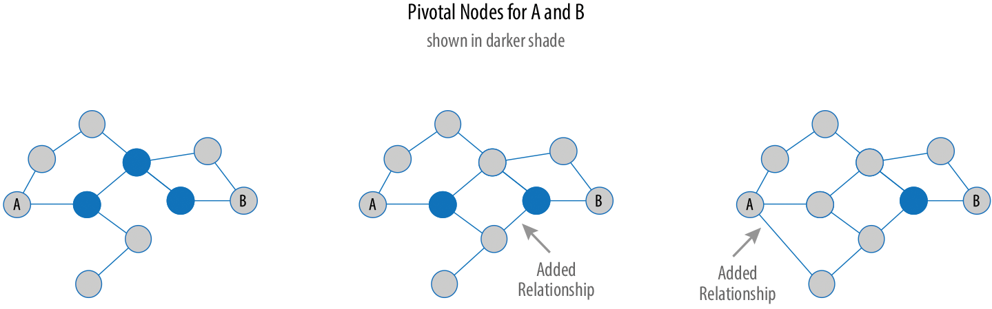
A node is considered pivotal for two other nodes if it lies on every shortest path between those nodes. Pivotal nodes play an important role in connecting other nodes—if you remove a pivotal node, the new shortest path for the original node pairs will be longer or more costly.
\(u\) is the node for which the in betweenness centrality is calculated
\(P\) total number of shortest path for s and t
\(p(u)\) number of shortest paths between between s and t, and passing through u
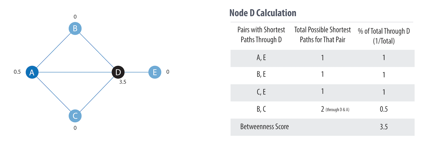
Illustration of the calulation of \(B(D)\)
Example use cases include:
Identifying influencers in various organizations.Powerful individuals are not necessarily in management positions, but can be found in “brokerage positions” using Betweenness Centrality. Removal of such influencers can seriously destabilize the organization.
Uncovering key transfer points in networks such as electrical grids. Counterintuitively, removal of specific bridges can actually improve overall robustness by “islanding” disturbances.
Helping microbloggers spread their reach on Twitter, with a recommendation engine for targeting influencers.
CALL gds.betweenness.stream({nodeProjection: "User",relationshipProjection: "FOLLOWS"})
YIELD nodeId, score
RETURN gds.util.asNode(nodeId).id  AS user, score
ORDER BY score DESC;
which returns
user |
centrality |
|---|---|
Alice |
10.0 |
Doug |
7.0 |
Mark |
7.0 |
David |
1.0 |
Bridget |
0.0 |
Charles |
0.0 |
Michael |
0.0 |
Amy |
0.0 |
James |
0.0 |
These result illustrate what we already know: “Alice is the most important person in the graph”
Adding a short-circuit in the graph
For large graphs, exact centrality computation isn’t practical. The fastest known algorithm for exactly computing betweenness of all the nodes has a runtime proportional to the product of the number of nodes and the number of relationships.
Let’s add a new user “Claire” who binds the two graphs together
WITH ["James","Michael","Alice","Doug","Amy"] as existing_users
MATCh (existing:User) where existing.id in existing_users
MERGE (newuser:User {id:"Claire"})
MERGE (newuser)<-[:FOLLOWS]-(existing)
MERGE (newuser)-[:FOLLOWS]->(existing)
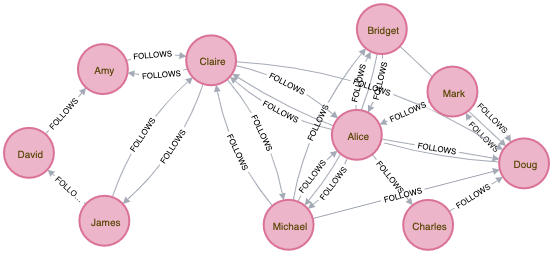
The impact of adding Claire as a “connection” is visible:
user |
centrality |
|---|---|
Claire |
44.33333333333333 |
Doug |
18.333333333333332 |
Alice |
16.666666666666664 |
Amy |
8.0 |
James |
8.0 |
Michael |
4.0 |
Mark |
2.1666666666666665 |
David |
0.5 |
Bridget |
0.0 |
Charles |
0.0 |
Let’s move on and delete the node “Claire”:
MATCH(n:User {id:"Claire"})
DETACH DELETE n
PageRank
Page Rank is an algorithm that measures the influence or importance of nodes in a
directed graph. It is computed by either iteratively distributing each node’s
score (originally based on degree) over its neighbours.
Theoretically this is equivalent traversing the graph in a random fashion and
counting the frequency of hitting each node during these walks.
PageRank (PR) is an algorithm used by Google Search to rank web pages in their search engine results. PageRank was named after Larry Page one of the founders of Google.
The intuition behind influence is that relationships to more important nodes contribute more to the influence of the node in question than equivalent connections to less important nodes.Measuring influence usually involves scoring nodes, often with weighted relationships, and then updating the scores over many iterations. Sometimes all nodes are scored, and sometimes a random selection is used as a representative distribution.
Formula for a node (page) \(u\) with \(n\) pages linking into this page. The pagerank \(PR(u)\) of this node is calculated as :
\(d\) is the dampening factor of 0.85 (default choice). This number between 0 and 1 is the probability that a user will continue without clicking. So which value does Google use then? Nobody outside the Google-complex knows, but the value recommended in the original paper is 0.85.
\(1-d\) is the probability that the node/page will be hit directly without any hit
\(PR(T_i)\) is the pagerank of node \(i\) (which connects to node \(u\))
\(CO(T_i)\) is the outdegree of a node \(i\)
T1,..Tn are called backlinks. These are all nodes that connect to the node node \(u\).
Iterative Procedure
PageRank is an iterative algorithm that runs either until scores converge or until a set number of iterations is reached.
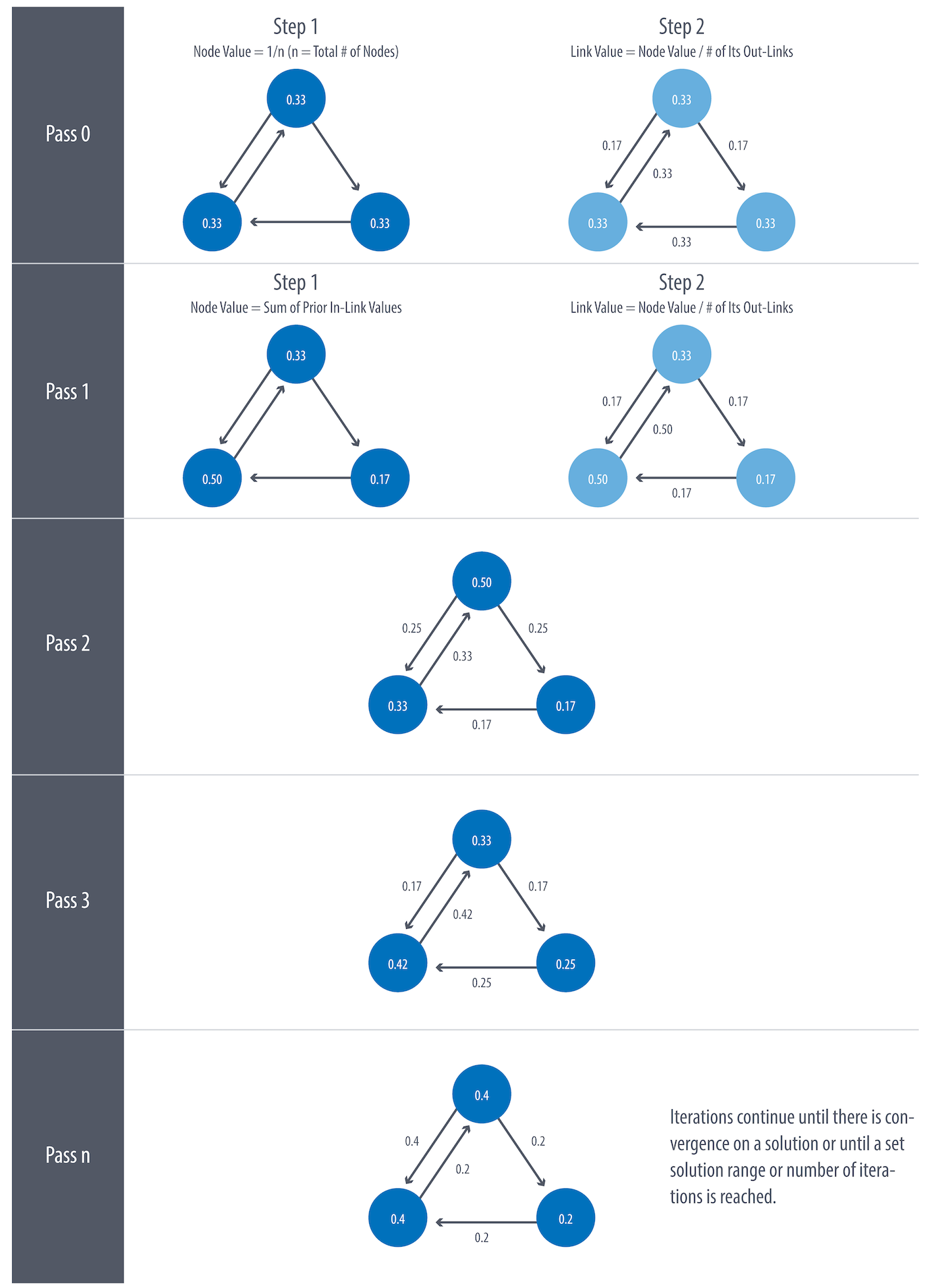
Without the use of the dampening factor, it could be possible to get stuck
in a so-called sink during the iteration procedure.
A node, or group of nodes, without outgoing relationships (also called a dangling node) can monopolize the PageRank score by refusing to share \(CO(T)=0\). This is known as a rank sink. You can imagine this as a surfer that gets stuck on a page, or a subset of pages, with no way out.
The damping factor provides another opportunity to avoid sinks by introducing a probability for direct link versus random node visitation. When you set d to 0.85, a completely random node is visited 15% of the time.
 CALL gds.pageRank.stream({  nodeProjection: "User",
relationshipProjection: "FOLLOWS",  maxIterations: 20,  dampingFactor: 0.85})
YIELD nodeId, score
RETURN gds.util.asNode(nodeId).id AS page, score
ORDER BY score DESC
LIMIT 5
Results :
page |
score |
|---|---|
Doug |
1.661536349568594 |
Mark |
1.5517852810554118 |
Alice |
1.1047215465462075 |
Bridget |
0.5332017140464881 |
Michael |
0.5332017140464881 |
Last change: Oct 30, 2023