Community Detection

The general principle in finding communities is that its members will have more relationships within the group than with nodes outside their group. Identifying these related sets reveals clusters of nodes, isolated groups, and network structure. This information helps infer similar behavior or preferences of peer groups, estimate resiliency, find nested relationships, and prepare data for other analyses.

Community detection algortihms are also called clustering and/or partitioning algorithms.

Community detection algorithms are also commonly used to produce network visualization for general inspection. The best known community detection algorithms are:

Overall Relationship Density of a Node / Network :

1. Triangle Count Coefficient

2. Clustering Coefficient

Finding Connected Clusters

3. Strongly Connected Components

4. Weakly Connected Components (see Lord of the Rings exercise)

Infer Clusters based on the spreading of labels

5. Label Propagation

Group Hierarchy

6. Louvain Modularity

Case Study: Python Dependencies

When managing Python environments, one of the key concerns is dependency management. Dependencies are all of the software components required by your project in order for it to work as intended and avoid runtime errors.

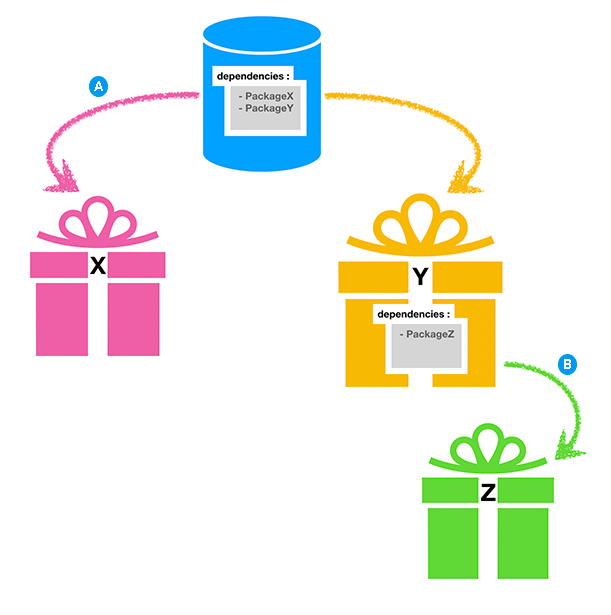
The data in this example is based on the dependencies between Python libraries. This kind of software dependency graph is used by developers to keep track of transitive interdependencies and conflicts in software projects.

You can download the data for the nodes and the relationships

WITH "file:///sw-nodes.csv" AS uri
LOAD CSV WITH HEADERS FROM uri AS row
MERGE (:Library {id: row.id});

WITH "file:///sw-relationships.csv" AS uri
LOAD CSV WITH HEADERS FROM uri AS row
MATCH (source:Library {id: row.src})
MATCH (destination:Library {id: row.dst})
MERGE (source)-[:DEPENDS_ON]->(destination);

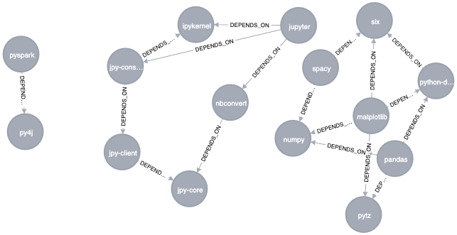
The result can be seen in the graph below. Looking at this graph, we see that there are three clusters of libraries. We can use visualizations on smaller datasets as a tool to help validate the clusters derived by community detection algorithms.

Measuring Algorithms

The two measuring algos are illustrated in the chart below:

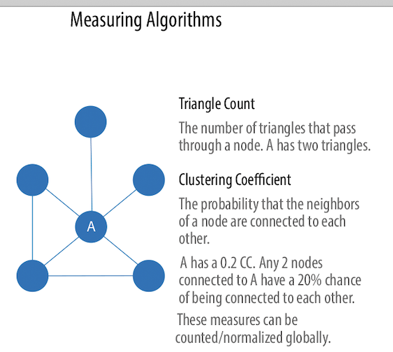
Triangle Count

Triangle Count determines the number of triangles passing through each node in the graph. A triangle is a set of three nodes, where each node has a relationship to all other nodes. Triangle Count can also be run globally for evaluating our overall dataset. NoteNetworks with a high number of triangles are more likely to exhibit small-world structures and behaviors.

To obtain some general stats:

CALL gds.triangleCount.stats({
nodeProjection:"Library",
relationshipProjection:  {DEPENDS_ON: {
type: "DEPENDS_ON",
   orientation: "UNDIRECTED"
 }}
})
YIELD globalTriangleCount,nodeCount

Note

nodeProjection enables the mapping of specific kinds of nodes into the in-memory graph. We can declare one or more node labels.

relationshipProjection enables the mapping of relationship types into the in-memory graph. We can declare one or more relationship types along with direction and properties.

globalTriangleCount	nodeCount
2	15

To visualise the triangles:

CALL gds.triangleCount.stream({
nodeProjection:"Library",
relationshipProjection:  {DEPENDS_ON: {
type: "DEPENDS_ON",
   orientation: "UNDIRECTED"
 }}
})
YIELD nodeId , triangleCount

RETURN gds.util.asNode(nodeId).id as package ,triangleCount as nbr_triangles
ORDER BY triangleCount DESC
LIMIT 8

package	nbr_triangles
jpy-console	1
python-dateutil	1
six	1
jupyter	1
ipykernel	1
matplotlib	1
pyspark	0
numpy	0

A call to the following procedure will calculate the triangles in the graph:

CALL gds.alpha.triangles({
nodeProjection: "Library",
relationshipProjection:  {
    DEPENDS_ON: {type: "DEPENDS_ON",
    orientation: "UNDIRECTED"}
    }
    })
 YIELD nodeA, nodeB, nodeC
 RETURN gds.util.asNode(nodeA).id AS nodeA,
        gds.util.asNode(nodeB).id AS nodeB,
        gds.util.asNode(nodeC).id AS nodeC;

nodeA	nodeB	nodeC
six	python-dateutil	matplotlib
jupyter	jpy-console	ipykernel

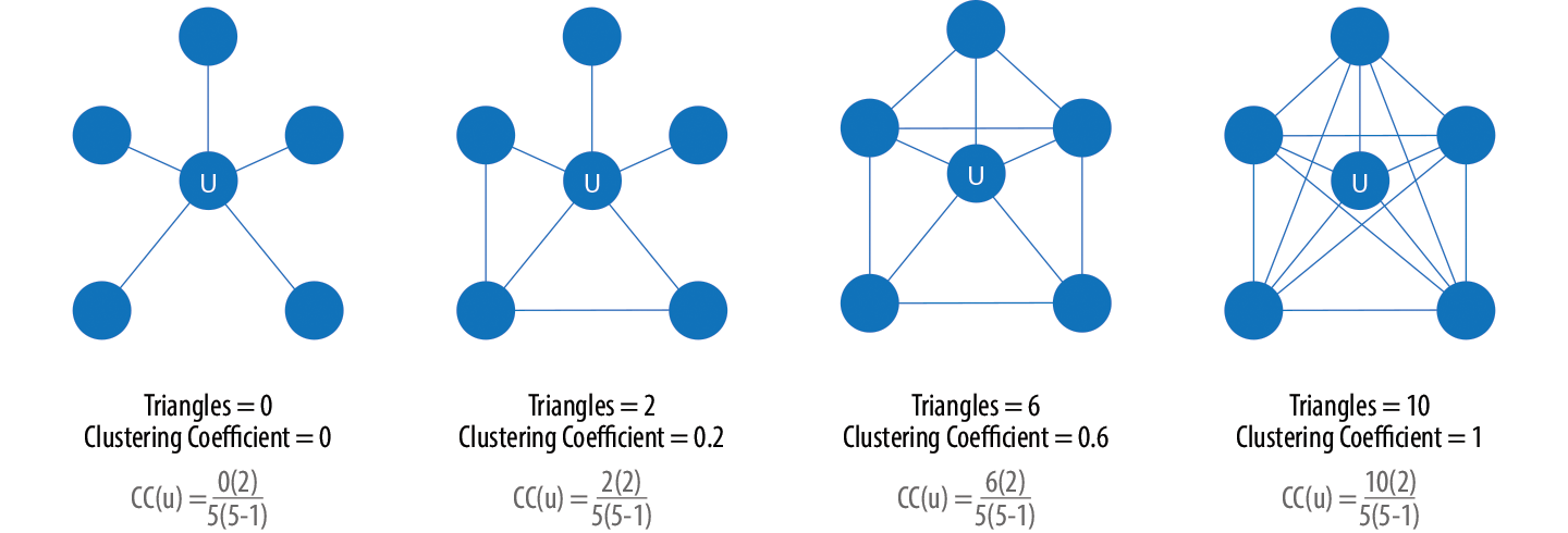
Clustering Coefficient

The goal of the Clustering Coefficient algorithm is to measure how tightly a group is clustered compared to how tightly it could be clustered. The algorithm uses Triangle Count in its calculations, which provides a ratio of existing triangles to possible relationships. A maximum value of 1 indicates a clique where every node is connected to every other node.

There are two types of clustering coefficients: local clustering and global clustering.

Local Clustering

The formula for the calculation of the local clustering coefficient is :

\[CC(u) = \frac{2 \times T_u}{D_u(D_u-1)}\]

Where :

• \(CC(u)\) is the calculated local clustering coefficient for node unsplash

• \(T_u\) is the number of triangles passing through the node

• \(D_u\) is the degree of the node

Global clustering

The global clustering coefficient is the normalized sum of the local clustering coefficients.

 CALL gds.localClusteringCoefficient.stream({
nodeProjection: "Library",
relationshipProjection:  {
  DEPENDS_ON: {
    type: "DEPENDS_ON",
    orientation: "UNDIRECTED"
  }
}
})
 YIELD nodeId, localClusteringCoefficient
WHERE localClusteringCoefficient > 0
RETURN gds.util.asNode(nodeId).id AS library, localClusteringCoefficient
ORDER BY localClusteringCoefficient DESC;

library	localClusteringCoefficient
ipykernel	1.0
six	0.3333333333333333
python-dateutil	0.3333333333333333
jupyter	0.3333333333333333
jpy-console	0.3333333333333333
matplotlib	0.16666666666666666

When to use ?

Clustering Coefficient can provide the probability that randomly chosen nodes will be connected. You can also use it to quickly evaluate the cohesiveness of a specific group or your overall network. Together these algorithms are used to estimate resiliency and look for network structures.

Strongly Connected Components (SCC)

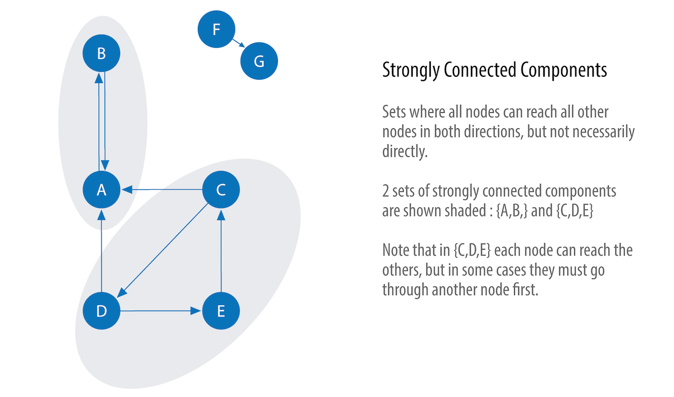
SCC finds sets of connected nodes in a directed graph where each node is reachable in both directions from any other node in the same set.

In Figure above you can see that the nodes in an SCC group don’t need to be immediate neighbors, but there must be directional paths between all nodes in the set.

When Should to use? Use as an early step in graph analysis to see how a graph is structured or to identify tight clusters that may warrant independent investigation. A component that is strongly connected can be used to profile similar behavior or inclinations in a group for applications such as recommendation engines.

 CALL gds.alpha.scc.stream({
nodeProjection: 'Library',
relationshipProjection: 'DEPENDS_ON'
})
YIELD nodeId, componentId
RETURN gds.util.asNode(nodeId).id AS Name, componentId AS Component
ORDER BY Component DESC

Name	Component
jpy-core	14
jpy-client	13
ipykernel	12
nbconvert	11
jpy-console	10
jupyter	9
py4j	8
spacy	7
matplotlib	6
pyspark	5
pytz	4
python-dateutil	3
numpy	2
pandas	1
six	0

So far the algorithm has only revealed that our Python libraries are very well behaved, but let’s create a circular dependency in the graph to make things more interesting. This should mean that we’ll end up with some nodes in the same partition.

MATCH (py4j:Library {id: "py4j"})
MATCH (pyspark:Library {id: "pyspark"})
MERGE (extra:Library {id: "extra"})
MERGE (py4j)-[:DEPENDS_ON]->(extra)
MERGE (extra)-[:DEPENDS_ON]->(pyspark);

Now if we run the SCC algorithm again we’ll see a slightly different result:

Name	Component
jpy-core	14
jpy-client	13
ipykernel	12
nbconvert	11
jpy-console	10
jupyter	9
spacy	7
matplotlib	6
pyspark	5
py4j	5
extra	5
pytz	4
python-dateutil	3
numpy	2
pandas	1
six	0

Connected Components

The Connected Components algorithm (or Weakly Connected Components) finds sets of connected nodes in an undirected graph where each node is reachable from any other node in the same set. It differs from the SCC algorithm because it only needs a path to exist between pairs of nodes in one direction, whereas SCC needs a path to exist in both directions.

Make it a habit to run Connected Components to test whether a graph is connected as a preparatory step for general graph analysis. Performing this quick test can avoid accidentally running algorithms on only one disconnected component of a graph and getting incorrect results.

 CALL gds.wcc.stream({
nodeProjection: "Library",
relationshipProjection: "DEPENDS_ON"
})
YIELD nodeId, componentId
RETURN componentId, collect(gds.util.asNode(nodeId).id) AS libraries
ORDER BY size(libraries) DESC;

componentId	libraries
0	[six,pandas,numpy,python-dateutil,pytz,matplotlib,spacy]
9	[jupyter,jpy-console,nbconvert,ipykernel,jpy-client,jpy-core]
5	[pyspark,py4j,extra]

Label Propagation

Both of the community detection algorithms that we’ve covered so far are deterministic: they return the same results each time we run them. The next two algorithms are examples of nondeterministic algorithms, where we may see different results if we run them multiple times, even on the same data.

The Label Propagation algorithm (LPA) is a fast algorithm for finding communities in a graph. In LPA, nodes select their group based on their direct neighbors. This process is well suited to networks where groupings are less clear and weights can be used to help a node determine which community to place itself within. It also lends itself well to semisupervised learning because you can seed the process with preassigned, indicative node labels.

There are two variations of Label Propagation (LPA)

• a (simple) push method

• the more typical pull method that relies on relationship weights.

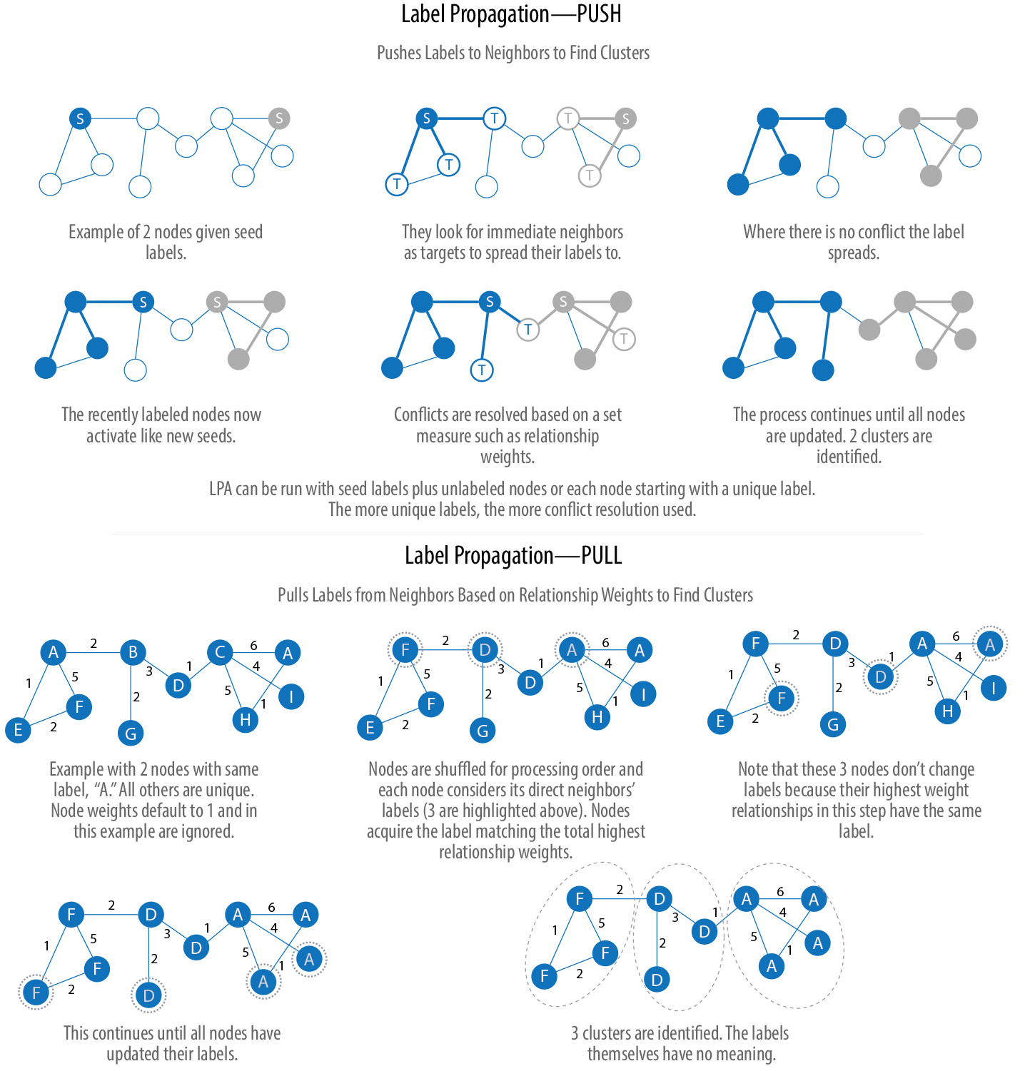
The steps often used for the Label Propagation pull method are:

1. Every node is initialized with a unique label (an identifier), and, optionally preliminary “seed” labels can be used.

2. These labels propagate through the network.

3. At every propagation iteration, each node updates its label to match the one with the maximum weight, which is calculated based on the weights of neighbor nodes and their relationships. Ties are broken uniformly and randomly.

4. LPA reaches convergence when each node has the majority label of its neighbors.

5. As labels propagate, densely connected groups of nodes quickly reach a consensus on a unique label. At the end of the propagation, only a few labels will remain, and nodes that have the same label belong to the same community.

CALL gds.labelPropagation.stream({
nodeProjection: "Library",
relationshipProjection: "DEPENDS_ON",
maxIterations: 10
})
YIELD nodeId, communityId
RETURN communityId AS label,
 collect(gds.util.asNode(nodeId).id) AS libraries
ORDER BY size(libraries) DESC;

label	libraries
0	[six,pandas,python-dateutil,matplotlib,spacy]
12	[jupyter,jpy-console,ipykernel]
14	[nbconvert,jpy-client,jpy-core]
15	[pyspark,extra]
2	[numpy]
4	[pytz]
8	[py4j]

Louvain Modularity

The Louvain algorithm is one of the fastest modularity-based algorithms. Louvain quantifies how well a node is assigned to a group by looking at the density of connections within a cluster in comparison to an average or random sample. As opposed to just looking at the concentration of connections within a cluster, this method compares relationship densities in given clusters to densities between clusters. The measure of the quality of those groupings is called modularity.

Networks with high modularity have dense connections between the nodes within modules but sparse connections between nodes in different modules. Modularity is often used in optimization methods for detecting community structure in networks. However, it has been shown that modularity suffers a resolution limit and, therefore, it is unable to detect small communities.

Note

Calculating Modularity

Imagine a network with \(n_c\) groups the Modularity of the network \(M\) is given by:

\[M = \sum_{c=1}^{n_c} M_c\]

where

\[M_c = [\frac{L_c}{L} - (\frac{k_c}{2L})^2]\]

As a consequence \(M_c \in [-1,1]\)

with

• \(L\) = the total number of connections on the network

• \(L_c\) = the total number of connections in the group (partition) c

• \(k_c\) = the total degree of the group (partition) c

In layman’s terms :

\(\frac{L_c}{L}\) is the fraction of relationships in the partition compared to all the partitions.

\((\frac{k_c}{2L})^2\) is the expected fraction if the relationships were distributed at random between the nodes.

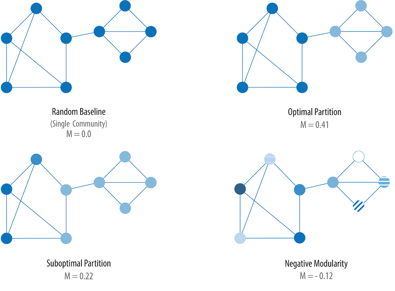
As an exampe calculate the modularity of the network (in two partitions) at the top of the Figure above:

• The dark partition \((\frac{7}{13}- (\frac{15}{2 \times 13})^2) = 0.205\)

• The light partition \((\frac{5}{13}- (\frac{11}{2 \times 13})^2) = 0.206\)

Adding the two together gives a modularity M = 0.41

The Louvain algorithm is a method with local maximization of the modularity. The partitioning of the graph is such to obtain maximum modularity.

Use Louvain Modularity to find communities in vast networks. This algorithm applies a heuristic, as opposed to exact, modularity, which is computationally expensive. Louvain can therefore be used on large graphs where standard modularity algorithms may struggle.

 CALL gds.louvain.stream({
  nodeProjection: "Library",
  relationshipProjection: "DEPENDS_ON",
  includeIntermediateCommunities: true
})
YIELD nodeId, communityId, intermediateCommunityIds
RETURN gds.util.asNode(nodeId).id AS libraries,
     communityId, intermediateCommunityIds;

• nodeProjection

  Enables the mapping of specific kinds of nodes into the in-memory graph. We can declare one or more node labels.

• relationshipProjection

  Enables the mapping of relationship types into the in-memory graph. We can declare one or more relationship types along with direction and properties.

• includeIntermediateCommunities

  Indicates whether to write intermediate communities. If set to false, only the final community is persisted.

libraries	communityId	intermediateCommunityIds
six	2	[0,2]
pandas	2	[4,2]
numpy	2	[2,2]
python-dateutil	2	[0,2]
pytz	2	[4,2]
pyspark	15	[5,15]
matplotlib	2	[0,2]
spacy	2	[2,2]
py4j	15	[5,15]
jupyter	12	[14,12]
jpy-console	12	[14,12]
nbconvert	12	[14,12]
ipykernel	12	[12,12]
jpy-client	12	[14,12]
jpy-core	12	[14,12]
extra	15	[15,15]

The intermediateCommunityIds column describes the community that nodes fall into at two levels. The last value in the array is the final community and the other one is an intermediate community.

The numbers assigned to the intermediate and final communities are simply labels with no measurable meaning. Treat these as labels that indicate which community nodes belong to such as “belongs to a community labeled 0”, “a community labeled 4”, and so forth.

For example, matplotlib has a result of [3,5]. This means that matplotlib’s final community is labeled 5 and its intermediate community is labeled 3.

The communityId column returns the final community for each node.We can also store the final and intermediate communities using the write version of the algorithm and then query the results afterwards.

The following query will run the Louvain algorithm and store the list of communities in the communities property on each node:

We can also store the final and intermediate communities using the write version of the algorithm and then query the results afterwards.

The following query will run the Louvain algorithm and store the list of communities in the communities property on each node:

CALL gds.louvain.write({
 nodeProjection: "Library",
 relationshipProjection: "DEPENDS_ON",
 includeIntermediateCommunities: true,
 writeProperty: "communities"
});

And the following query will run the Louvain algorithm and store the final community in the finalCommunity property on each node:

CALL gds.louvain.write({
 nodeProjection: "Library",
 relationshipProjection: "DEPENDS_ON",
 includeIntermediateCommunities: false,
 writeProperty: "finalCommunity"
});

Once we’ve run these two procedures, we can write the following query to explore the final clusters:

MATCH (l:Library)
RETURN l.finalCommunity AS community, collect(l.id) AS libraries
ORDER BY size(libraries) DESC;

community	libraries
2	[six,pandas,numpy,python-dateutil,pytz,matplotlib,spacy]
12	[jupyter,jpy-console,nbconvert,ipykernel,jpy-client,jpy-core]
15	[pyspark,py4j,extra]

This clustering is the same as we saw with the connected components algorithm.

matplotlib is in a community with pytz, spacy, six, pandas, numpy, and python-dateutil.

An additional feature of the Louvain algorithm is that we can see the intermediate clustering as well. The following query will show us finer-grained clusters than the final layer did:

community	libraries
14	[jupyter,jpy-console,nbconvert,jpy-client,jpy-core]
0	[six,python-dateutil,matplotlib]
4	[pandas,pytz]
2	[numpy,spacy]
5	[pyspark,py4j]
12	[ipykernel]
15	[extra]

Last change: Oct 30, 2023