Graph Datascience Library in Neo4j¶

The Neo4j GDS Library provides data scientists with a rich toolkit offering a flexible, analytics-designed data structure for global computations, and a library of parallelized, algorithms that quickly compute over very large graphs. Graph algorithms are unsupervised machine learning methods and heuristics that learn and describe the topology of your graph and are highly parallelized to quickly compute results over tens of billions of nodes.

General Info

Introduction¶

The Neo4j Graph Data Science library is available in two editions.

The open source Community Edition includes all algorithms and features, but is limited to four CPU cores.
The Neo4j Graph Data Science library Enterprise Edition can run on an unlimited amount of CPU cores.

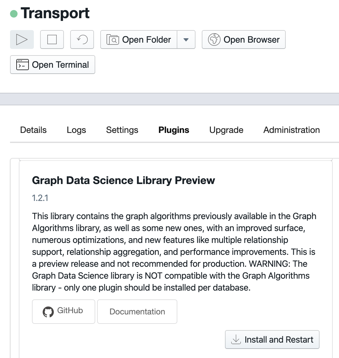
Installation¶

The Neo4j Graph Data Science (GDS) library is delivered as a plugin to the Neo4j Graph Database. The plugin needs to be installed into the database.

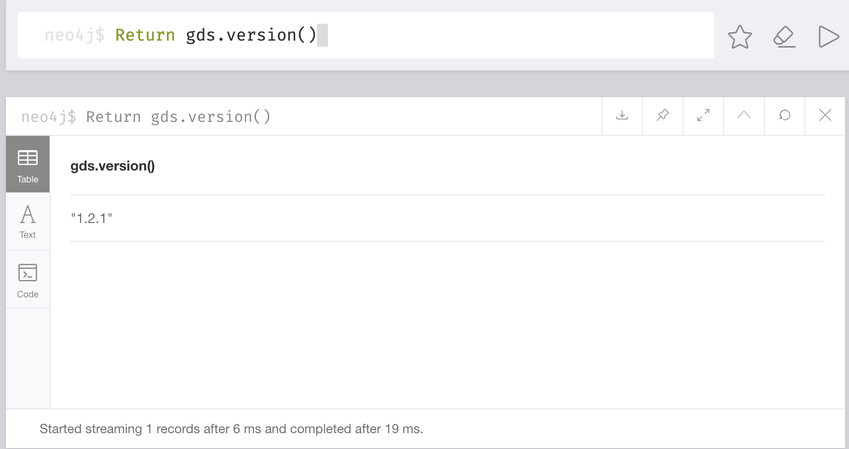
To verify your installation, the library version can be printed by entering into the browser:

RETURN gds.version()

Overview¶

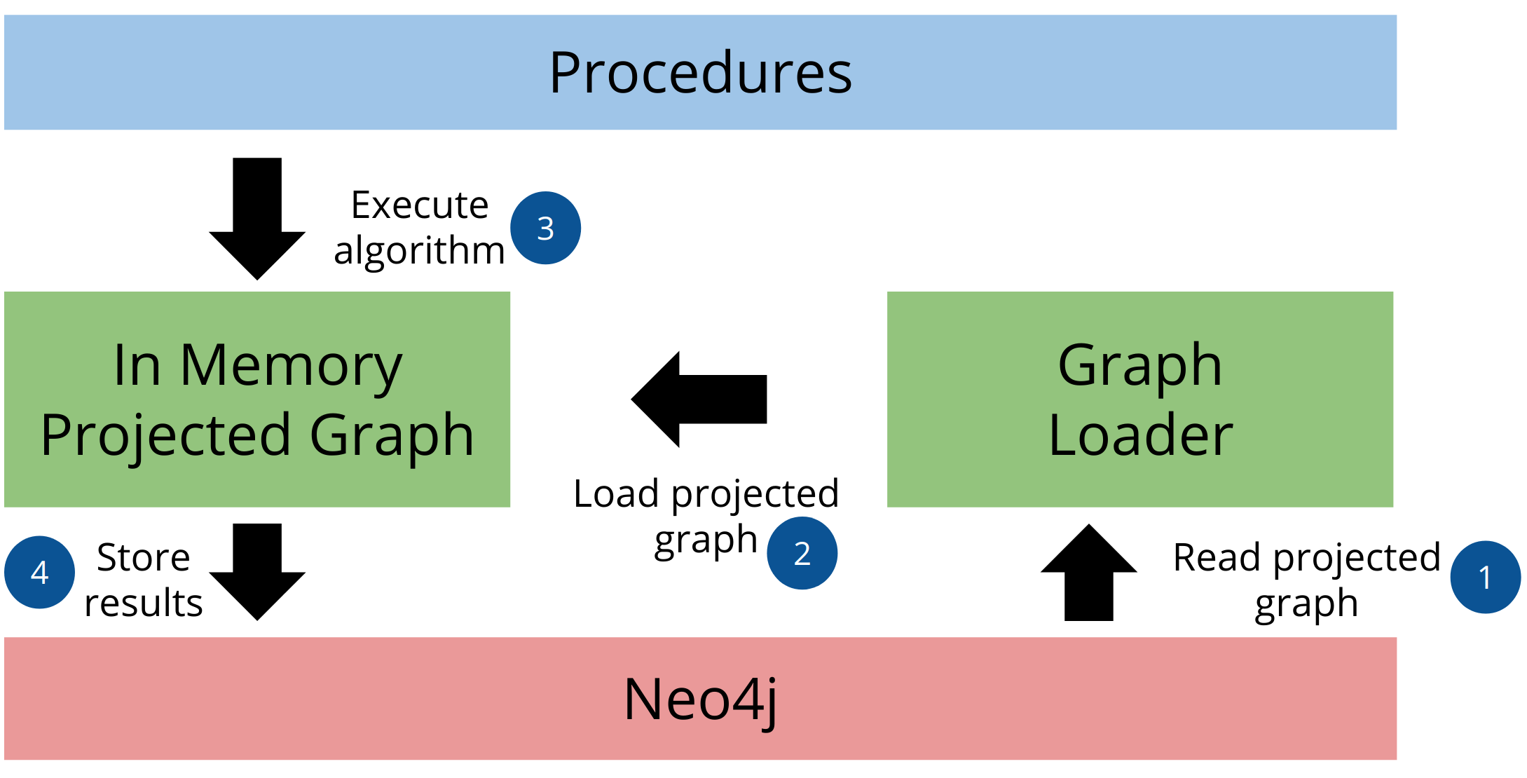
In order for any algorithm in the GDS library to run, we must first create a graph to run on. The graph is created as either an anonymous graph or a named graph. An anonymous graph is created for just a single algorithm and will be lost after its execution has finished. A named graph is given a name and stored in the graph catalog.

Graph Management¶

Estimating memory¶

In many use cases it will be useful to estimate the required memory of a graph and an algorithm before running it in order to make sure that the workload can run on the available hardware. To make this process easier every algorithm supports the .estimate mode, which returns an estimate of the amount of memory required to run graph algorithms.

If the estimation check can determine that the current amount of free memory is insufficient to carry through the operation, the operation will be aborted and an error will be reported. The error will contain details of the estimation and the free memory at the time of estimation.

This heap control logic is restrictive in the sense that it only blocks executions that are certain to not fit into memory. It does not guarantee that an execution that passed the heap control will succeed without depleting memory. Thus, it is still useful to first run the estimation mode before running an algorithm or graph creation on a large data set, in order to view all details of the estimation.

Some graph catalog function¶

gds.graph.create :Creates a graph in the catalog using a Native projection.
gds.graph.create.cypher: Creates a graph in the catalog using a Cypher projection.
gds.graph.list: Prints information about graphs that are currently stored in the catalog.
gds.graph.exists: Checks if a named graph is stored in the catalog.
gds.graph.removeNodeProperties: Removes node properties from a named graph.
ds.graph.deleteRelationships: Deletes relationships of a given relationship type from a named graph.
gds.graph.drop: Drops a named graph from the catalog.
gds.graph.writeNodeProperties: Writes node properties stored in a named graph to Neo4j.
gds.graph.writeRelationship: Writes relationships stored in a named graph to Neo4j.
gds.beta.graph.export`: Exports a named graph into a new offline Neo4j database.

Running algorithms¶

All algorithms are exposed as Neo4j procedures. They can be called directly from Cypher using Neo4j Browser, cypher-shell, or from your client code using a Neo4j Driver in the language of your choice.

There are 4 different execution models to run algos:

stream : returns results

The stream mode will return the results of the algorithm computation as Cypher result rows. The returned data can be a node ID and a computed value for the node (such as a Page Rank score, or WCC componentId), or two node IDs and a computed value for the node pair (such as a Node Similarity similarity score).

Note: If the graph is very large, the result of a stream mode computation will also be very large. Using the ORDER BY and LIMIT subclauses in the Cypher query is always a good idea.
write : write results in DB

The write mode will write the results of the algorithm computation back to the Neo4j database. This is the only execution mode that will make any modifications to the Neo4j database.

The written data can be:
- node properties (such as Page Rank scores)
- new relationships (such as Node Similarity similarities)
- relationship properties
mutate : change inmemory graph

The mutate mode is very similar to the write mode but instead of writing results to the Neo4j database, they are made available at the in-memory graph.
stats : returns statistical results for the algorithm computation

The stats mode returns statistical results for the algorithm computation like counts or a percentile distribution.

The different algorithms are called on a graph using the name of the graph as argument. The code below runs the wcc algorithm on "my_graph". The Weakly Connected Components (wcc), or Union Find, algorithm finds sets of connected nodes in an undirected graph where each node is reachable from any other node in the same set.

CALL gds.wcc.stream('my_graph')
YIELD nodeId, componentId
RETURN componentId, count(*) as size

The requested output is populated using the YIELD argument.

componentId = Id of the componentId
nodeId = Id of the node

The available outputs depend on the execution model and the algorithm. YIELD retrieves the different outputs.

Graph Catalog¶

The graph catalog is a concept within the GDS library that allows managing multiple graph projections by name. Using that name, a created graph can be used many times in the analytical workflow.

Note

Graph Projections: Graph algorithms run on a graph data model which is a projection of the Neo4j property graph data model. A graph projection can be seen as a view over the stored graph, containing only analytical relevant, potentially aggregated, topological and property information. Graph projections are stored entirely in-memory using compressed data structures optimized for topology and property lookup operations.

The graph catalog is a concept within the GDS library that allows managing multiple graph projections by name. Using that name, a created graph can be used many times in the analytical workflow.

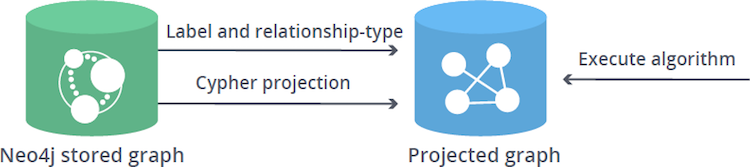
There are two variants of projecting a graph from the Neo4j database into main memory:

Native projection Provides the best performance by reading from the Neo4j store files. Recommended to be used during both the development and the production phase.
Cypher projection The more flexible, expressive approach with lesser focus on performance. Recommended to be primarily used during the development phase.

Our First Algorithm¶

In this example we will use a data-set on Lord of the Rings made available by José Calvo. Much of the code comes from a blog.

The dataset describes interactions between persons, places, groups, and things. Which leaves us with the following Node-labels:

Person
Place
Group
Thing

We store interactions from each book as a separate relationship, meaning that the interactions from the first book will be saved as the INTERACTS_1 relationships, second book interactions as INTERACTS_2, and so on. Keep in mind that we will treat interaction relationships as undirected and weighted.

Create a new database in your existing DBMS :

CREATE DATABASE LordoftheRing

Creating the nodes

The nodes are stored into a csv file (https://raw.githubusercontent.com/morethanbooks/projects/master/LotR/ontologies/ontology.csv)

id	type	Label	FreqSum	subtype	gender
andu	pla	Anduin	109	pla
arag	per	Aragorn	1069	men	male
arat	per	Arathorn	36	men	male
arwe	per	Arwen	51	elves	female
bage	pla	Bag End	77	pla
bali	per	Balin	30	dwarf	male
bere	per	Beregond	77	men	male

LOAD CSV WITH HEADERS FROM "https://raw.githubusercontent.com/morethanbooks/projects/master/LotR/ontologies/ontology.csv" as row
FIELDTERMINATOR "\t"
WITH row, CASE row.type WHEN 'per' THEN 'Person'
                     WHEN 'gro' THEN 'Group'
                     WHEN 'thin' THEN 'Thing'
                     WHEN 'pla' THEN 'Place' END as label
CALL apoc.create.nodes(['Node',label], [apoc.map.clean(row,['type','subtype'],[null,""])]) YIELD node
WITH node, row.subtype as class
MERGE (c:Class{id:class})
MERGE (node)-[:PART_OF]->(c)

The number of labels created:

CALL apoc.meta.stats() YIELD labels
RETURN labels

The number of nodes for the different combinations of labels:

MATCH (n)
RETURN DISTINCT count(labels(n)), labels(n);

count(labels(n))	labels(n)
24	[Node,Place]
43	[Node,Person]
7	[Node,Group]
1	[Node,Thing]
11	[Class]

Note how we used the function apoc.create.nodes to create nodes with dynamic labels This function has the following signature: ‘apoc.create.nodes([‘Label’], [{key:value,…}])’
Each line in the csv file is used twice. The apoc.create.nodes has indeed two arguments : [‘Node’,label].
- The first argument creates a Node
- The second creates a node with a label from the list: Person, Place, Group or Thing
Each node has the following properties : id, Label, FreqSum and gender This is a result of the apoc.map.clean function which removed the column type and subtype.

The gender column is also removed when it is null or empty (as this is the case for Place-nodes)
The csv-file uses tabs (“\t”) as separator.
Do you understand why we used MERGE in the final two lines of the code ?

MERGE (c:Class{id:class})

MERGE (node)-[:PART_OF]->(c)

The first line in the CSV file is the river Anduin described in the book Lord of the Rings:

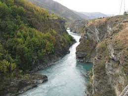
Anduin river¶

MATCH (n:Node {id:"andu"})
MATCH (m:Place {id:"andu"})
return n,m

Returns :

n	m
{Label:Anduin,FreqSum:109,id:andu}	{Label:Anduin,FreqSum:109,id:andu}

Creating the relationships (for the 3 books)

The three volumes were titled The Fellowship of the Ring, The Two Towers and The Return of the King. In each of the books there is a relationship which we are going to study:

The relationship (undirected) are stored in csv files. But unfortunately the structure of the different csv files is different. For book 3, Source is used instead of IdSource.

IdSource	IdTarget	Weight	Type
frod	sams	171	undirected
frod	ganda	129	undirected
arag	frod	105	undirected
bilb	frod	96	undirected
frod	pipp	80	undirected
pipp	sams	72	undirected
frod	ring	71	undirected
frod	merr	64	undirected
frod	shir	64	undirected
merr	pipp	57	undirected

The relation between Gandalf and Frodo has a weight of 129. A data-scientist has counted how many times those two persons appear in the same paragraph. This occurence determines the weight of the relation.

Frodo: …I wish the Ring had never come to me… I wish none of this had happened. Gandalf: …So do all who live to see such times; but that is not for them to decide. All we have to decide is what to do with the time that is given to us…¶

UNWIND ['1','2','3'] as book
LOAD CSV WITH HEADERS FROM "https://raw.githubusercontent.com/morethanbooks/projects/master/LotR/tables/networks-id-volume" + book + ".csv" AS row
MATCH (source:Node{id:coalesce(row.IdSource,row.Source)})
MATCH (target:Node{id:coalesce(row.IdTarget,row.Target)})
CALL apoc.create.relationship(source, "INTERACTS_" + book,
         {weight:toInteger(row.Weight)}, target) YIELD rel
RETURN distinct true

Note the use of COALESCE(). This function has its roots in SQL. In SQL the COALESCE function accepts a list of parameters, returning the first non-Null value from the list:

COALESCE(value1, value2, value3, …)

Will return value1 as long as this is not null
Otherwise it will return value2 as long as this one is not null
etc…

It allows to have a fallback default value when a property doesn’t exist on a node or relationship. Or we may want to perform an equality or inequality comparison against a possible null value, and use a default if the value happens to be null.

This gives us an elegent way to deal with the different versions of the CSV files.

The code-above also makes use of the function apoc.create.relationship to create a relationship between two nodes. The code-snippet below illustrates the syntax of this apoc procedure. It requires two nodes (source and target), a string for the relation and a map to describe the properties (if any) between the two nodes:

MATCH (p:Person {name: "Tom Hanks"})
MATCH (m:Movie {title:"You've Got Mail"})
CALL apoc.create.relationship(p, "ACTED_IN", {roles:['Joe Fox']}, m)
YIELD rel
RETURN rel;

Carve out what you want.¶

The graph contains 75 Nodes split across the following labels:

Place: 24

Person : 43

Group : 7

Thing : 1

The number of relationship equals 2299 spread across the three books :

Book1 : 758 (“INTERACTS_1”)
Book2 : 780 (“INTERACTS_2”)
Book3 : 686 (“INTERACTS_3”)
All Books : 75 (“PART_OF”)

Now is the time to create our own graphs (on which we will apply algorithms) and add these to the Graph Catalog.

The syntax to add a named graph to the Graph Catalog is:

CALL gds.graph.create(graph name, node label, relationship type

The code below adds the graph whole_graph to the Graph Catalog:

CALL gds.graph.create('whole_graph','*', '*')

In the next step, we want to ignore PART_OF relationships and only focus on INTERACTS_1,INTERACTS_2 or INTERACTS_3 relationships.

CALL gds.graph.create('all_interacts','Node',
  ['INTERACTS_1', 'INTERACTS_2', 'INTERACTS_3'])

The graphs in the catalog can be retrieved:

CALL gds.graph.list() YIELD graphName as name
return name

Before you run a graph algorithm, it is helpful to understand what the memory requirements will be for loading the data for the analysis, as well as the memory that will be required to run the algorithm. The estimate() function is used to provide you with this information and is available for the production-quality tier algorithms.

Lets determine the memory requirements for the wcc algorithm on the dataset we just created:

Part 1: Determine the memory requirements for loading our named graphs.

Imagine you want to create a graph with the node Person exclusively for the relationship INTERACTS_1:
```
CALL gds.graph.create.estimate('Person', 'INTERACTS_1')
YIELD requiredMemory
```
Results in a required memory = “289 KiB”. This Cypher-script does not create the graph !

If you want to add the weight of the relationship:
```
CALL gds.graph.create.estimate('Person', 'INTERACTS_1',
{relationshipProperties:'weight'})
YIELD requiredMemory
```
results in a higher required memory requirement

To create this graph, the following Cypher code is required:
```
CALL gds.graph.create('MyGraph','Person',
'INTERACTS_1',{relationshipProperties:'weight'})
YIELD *
```
Part 2: Determine the memory requirements for running algorithms on these graphs.

In this case we want to run the wcc algorithm on one of the graphs. To check the required memory :
```
CALL gds.wcc.stream.estimate('all_interacts')
YIELD requiredMemory
```
Which results in a required memory of 792 Bytes.

On each of the graphs we just added to the catalog, we can now run the wcc algorithm. The Weakly Connected Components (WCC) algorithm is used to find disconnected subgraphs or islands within our network. WCC belongs the family of Community Detection Algorithms.

WCC is often used early in an analysis to understand the structure of a graph. Using WCC to understand the graph structure enables running other algorithms independently on an identified cluster. As a preprocessing step for directed graphs, it helps quickly identify disconnected groups.

CALL gds.wcc.stream('all_interacts') YIELD nodeId, componentId
RETURN componentId, count(*) as size,
   collect(gds.util.asNode(nodeId).Label) as ids
ORDER BY size DESC LIMIT 10

Which results in :

componentId	size	ids
0	73	[Anduin,…..]
26	1	[Mirkwood]
25	1	[Old Forest]

The graph-projection has one component with a lot of Nodes and two tiny components consisting of only a single node. We can conclude that the Nodes Mirkwood and Old Forest have no INTERACTS_1,INTERACTS_2 or INTERACTS_3 relationships.

The following cypher script allows you to check this:

UNWIND ['Mirkwood','Old Forest'] as lbl
MATCH (n:Node)
MATCH (n:Node)
WHERE n.Label = lbl
WITH n
MATCH (n)-[]-(m)
RETURN n,m

Our projection can be refined using a filter such that we only use the relationships from the first book (INTERACTS_1 relationships).

CALL gds.wcc.stream('all_interacts',
 {relationshipTypes:['INTERACTS_1']})
 YIELD nodeId, componentId
 RETURN componentId, count(*) as size,
    collect(gds.util.asNode(nodeId).Label) as ids
 ORDER BY size DESC LIMIT 10

componentId	size	ids
0	62	[Anduin,…]
21	1	[Ents]
26	1	[Mirkwood]
23	1	[Eorl]
24	1	[Éowyn]
25	1	[Old Forest]
22	1	[Éomer]
27	1	[Faramir]
38	1	[Gorbag]
6	1	[Beregond]

All the names that are alone in a component are Person,Places,… that have not been introduced in the first book.

Deleting our graph :

CALL gds.graph.drop('all_interacts')

Writing Node properties into a Neo4j Database¶

Imagine you have launched an algorithm on an in-memory graph. An algorithm which calculates a property for each of the nodes. You then might want to stored this value as a property in the database.

In the example belowe we create a test graph for all the Person nodes and calculated the wcc-algorithm.

The componentId result is stored as a new property in neo4j

CALL gds.graph.create('test','Person','*') Yield graphName
CALL gds.wcc.mutate('test',{mutateProperty:'componentId'}) Yield componentCount
CALL gds.graph.writeNodeProperties('test', ['componentId']) Yield propertiesWritten
RETURN  propertiesWritten

After running the code about, all the Person nodes in the database have a new property componentId

Writing Relationship (+ properties) into a Neo4j Database¶

Syntax :

CALL gds.graph.writeRelationship('name of graph',
                                 'name of relationship',
                                 'similarityScore')

Utility Functions¶

gds.util.asNodes() returns nodes with a given id

The code below makes a list of the person that have an interaction with frodo in the first book

MATCH (frodo:Person {id:'frod'})
MATCH (frodo)-[:INTERACTS_1]->(p:Person)
WITH collect(id(p)) AS id
RETURN id

This script returns an uncomprehensible array of ids. Utility functions will help us out :

MATCH (frodo:Person {id:'frod'})
MATCH (frodo)-[:INTERACTS_1]->(p:Person)
WITH collect(id(p)) AS id
RETURN [x in gds.util.asNodes(id)| x.id] AS nodeids

gds.util.nodeProperty returns a property from a node in a named graph

I Don’t want to write code¶

In this case you can use NEuler. This is a no-code user interface that helps users onboard with the Neo4j Graph Data Science Library.

It supports running each of the graph algorithms in the library, viewing the results, and also provides the Cypher queries to reproduce the results.

Neuler is also known as the The Graph Data Science Playground. It can be installed from the Graph Apps Gallery.

Last change: Oct 30, 2023