Pathfinding¶

History¶

Path finding has a long history, and is considered to be one of the classical graph problems; it has been researched as far back as the 19th century. It gained prominence in the early 1950s in the context of ‘alternate routing’, i.e. finding a second shortest route if the shortest route is blocked.

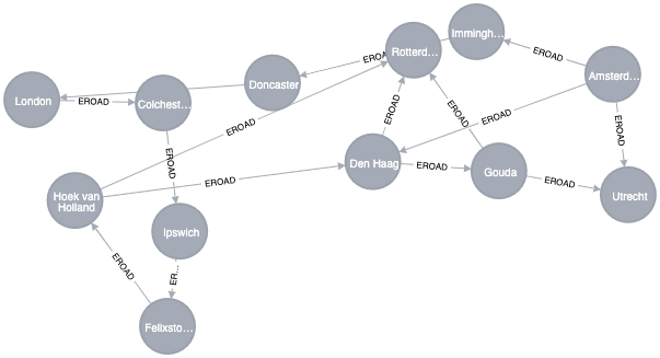
Dijkstra came up with his algorithm in 1956 while trying to come up with something to show off the new ARMAC computers. He needed to find a problem and solution that people not familiar with computing would be able to understand, and designed what is now known as Dijkstra’s algorithm. He later implemented it for a slightly simplified transportation map of 64 cities in the Netherlands.

Overview of the Paths¶

Overview of the pathfinding algorithms¶
Type	What it does	Example use
Shortest Path	Calculates the shortest path between a pair of nodes	Finding driving directions between two locations
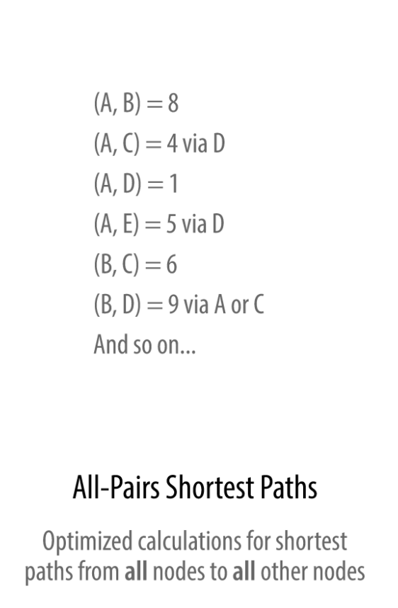
All Pairs Shortest Path	Calculates the shortest path between all pairs of nodes in the graph	Evaluating alternate routes around a traffic jam
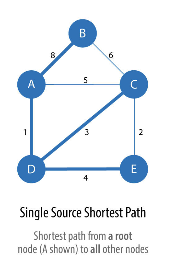
Single Source Shortest Path	Calculates the shorest path between a single root node and all other nodes	Least cost routing of phone calls
Minimum Spanning Tree	Calculates the path in a connected tree structure with the smallest cost for visiting all nodes	Optimizing connected routing, such as laying cable or garbage collection
Random Walk	Returns a list of nodes along a path of specified size by randomly choosing relationships to traverse.	Augmenting training for machine learning or data for graph algorithms.

Example Data: The Transport Graph¶

csv-file for the nodes (download)

csv_file for the connections between the cities (download)

Loading Nodes (Cities)

LOAD CSV WITH HEADERS FROM "file:///data_transport-nodes.csv"  AS row
MERGE (place:Place {id:row.id})
SET place.latitude = toFloat(row.latitude),
    place.longitude = toFloat(row.longitude),
    place.population = toInteger(row.population)

Creating the connections

LOAD CSV WITH HEADERS FROM "file:///data_transport-relationships.csv" as row
MATCH (origin:Place {id:row.src})
MATCH (destination:Place {id:row.dst})
MERGE (origin)-[:EROAD {distance: toInteger(row.cost)}]->(destination)

Graph Catalog¶

CALL gds.graph.create('myGraph','Place','EROAD',{relationshipProperties: 'distance'})

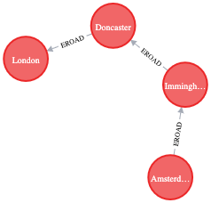
Shortest Path¶

The Shortest Path algorithm calculates the shortest (weighted) path between a pair of nodes.

Use Shortest Path to find optimal routes between a pair of nodes, based on either the number of hops or any weighted relationship value. For example, it can provide real-time answers about degrees of separation, the shortest distance between points, or the least expensive route. You can also use this algorithm to simply explore the connections between particular nodes.

Example use cases include:

Finding directions between locations (Google Maps)
Finding the degrees of separation between people in social networks.
Finding the number of degrees of separation between an actor and Kevin Bacon based on the movies they’ve appeared in (the Bacon Number). An example of this can be seen on the Oracle of Bacon website.
Calculation of the Erdos number of a mathenatician.

Note

You’ll notice in graph analytics the use of the terms weight, cost, distance, and hop when describing relationships and paths.

Weight is the numeric value of a particular property of a relationship.
Cost is used similarly, but we’ll see it more often when considering the total weight of a path.
Distance is often used within an algorithm as the name of the relationship property that indicates the cost of traversing between a pair of nodes.
Hop is commonly used to express the number of relationships between two nodes.

You may see some of these terms combined, as in “It’s a five-hop distance to London” or “That’s the lowest cost for the distance.”

MATCH (source:Place {id: 'Amsterdam'}), (target:Place {id: 'London'})
CALL gds.shortestPath.dijkstra.stream('myGraph', {
   sourceNode: source,
   targetNode: target,
   relationshipWeightProperty: 'distance'})
YIELD index, sourceNode, targetNode, totalCost, nodeIds, costs, path
RETURN index,
gds.util.asNode(sourceNode).name AS sourceNodeName,
gds.util.asNode(targetNode).name AS targetNodeName,
totalCost,
[nodeId IN nodeIds | gds.util.asNode(nodeId).name] AS nodeNames,
costs,
nodes(path) as path
ORDER BY index

All Pairs Shortest Paths¶

Shortest path from every node to every other node

Single Source Shortest Path¶

Minimum Spanning Tree¶

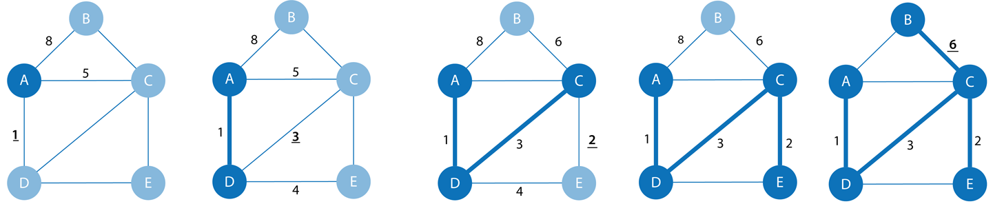
The Minimum (Weight) Spanning Tree algorithm starts from a given node and finds all its reachable nodes and the set of relationships that connect the nodes together with the minimum possible weight. It traverses to the next unvisited node with the lowest weight from any visited node, avoiding cycles.

The Minimum Spanning Tree algorithm operates as demonstrated in the figure below:

Use Minimum Spanning Tree when you need the best route to visit all nodes.